Note
Click here to download the full example code
StairAmbulationHealthy2021 - A Stride Segmentation and Event Detection dataset with focus on stairs#
The dataset can be downloaded from here:
Note
The dataset only contains the healthy participants of the full dataset presented in the paper!
General information#
The dataset was recorded with Nilspod V2 sensors from Portabiles. One sensor was attached on the instep of each foot and one sensor was attached on the lower back. On loading the transform the coordinate systems of the foot-mounted IMUs to the gaitmap coordinate system.

We provide two tpcp.Dataset classes to access the data:
StairAmbulationHealthy2021PerTest: This class allows to access all data and events for each of the performed gait tests individually.StairAmbulationHealthy2021Full: This class allows to access the entire recordings for each participant (two recordings per participant) independently of the performed gait tests.
In the following we will show the usage of both classes and the data that is contained within.
Warning
For this example to work, you need to have a global config set containing the path to the dataset.
Check the README.md for more information.
StairAmbulationHealthy2021PerTest#
First we can simply create an instance of the dataset class and directly see the contained data points. Note, that we will enable the loading of all available data (pressure, baro, and hip sensor). You might want to disable that, to reduce the RAM usage and speed up the data loading.
from joblib import Memory

from gaitmap_datasets import StairAmbulationHealthy2021PerTest

dataset = StairAmbulationHealthy2021PerTest(
    include_pressure_data=True,
    include_baro_data=True,
    include_hip_sensor=True,
    memory=Memory("../.cache"),
)
dataset
We can see that we have 20 participants and each of them has performed 26 gaittests on different level walking and stair configurations. For more information about the individual tests see the documentation of the dataset itself.
Using the dataset class, we can select any subset of tests and participants.
subset = dataset.get_subset(
    test=["stair_long_down_normal", "stair_long_up_normal"], participant=["subject_01", "subject_02"]
)
subset
Once we have the selection of data we want to work with, we can iterate the dataset object to access the data of individual datapoints or just index it as below.
On this datapoint, we can now access the data. We will start with the metadata. It contains all the general information about the participant and the sensors.
{'subject_id': '001', 'gender': 'm', 'age': 30, 'height': 180, 'weight': 80, 'shoe_size': 43, 'sensor_ids': {'left_sensor': '6f13', 'right_sensor': '48b4', 'hip_sensor': '7fe5'}, 'fsr_ids': {'left_sensor': {'toe': {'id': 11, 'r_ref': 960}, 'mth': {'id': 12, 'r_ref': 1080}, 'heel': {'id': 14, 'r_ref': 1600}}, 'right_sensor': {'toe': {'id': 25, 'r_ref': 960}, 'mth': {'id': 23, 'r_ref': 1040}, 'heel': {'id': 13, 'r_ref': 1750}}}}
We can also access the imu data, the pressure data and the barometer data. All of them have an index that marks the seconds from the start of the individual test we selected.
In addition we provide ground truth information for the event detection. All event data is provided in samples from the start of the test.
Note that we use a trailing _ to indicate that this is data calculated based on the ground truth and not just the
IMU data.
First, manually labeled stride borders.
segmented_stride_list = datapoint.segmented_stride_list_
segmented_stride_list["left_sensor"]
Second, the events extracted using the pressure-insole.
Note, that the min_vel event is actually calculated based on the IMU data.
For more information see the docstring of this property.
insole_events = datapoint.pressure_insole_event_list_
insole_events["left_sensor"]
As further groundtruth we provide a label for each segmented stride that contains information about the height change during the stride. This information is derived by measuring the heights of the individual stair steps and labeling each stride based on video, to mark all strides that were performed on a specicic stair configuration.
{'left_sensor':        start     end        type  z_level
s_id
589    318.0   567.0       level      0.0
591    567.0   788.0  descending    -29.0
593    788.0   996.0  descending    -29.0
595    996.0  1204.0  descending    -29.0
597   1204.0  1411.0  descending    -29.0
599   1411.0  1619.0  descending    -29.0
601   1619.0  1832.0  descending    -29.0
603   1832.0  2061.0  descending    -29.0
605   2061.0  2279.0  descending    -14.5
607   2279.0  2473.0  descending    -29.0
609   2473.0  2673.0  descending    -29.0
611   2673.0  2869.0  descending    -29.0
613   2869.0  3070.0  descending    -29.0
615   3070.0  3269.0  descending    -29.0
617   3269.0  3483.0  descending    -29.0
619   3483.0  3714.0  descending    -29.0
621   3714.0  3969.0       level      0.0, 'right_sensor':        start     end        type  z_level
s_id
588    169.0   450.0       level      0.0
590    450.0   682.0  descending    -14.5
592    682.0   895.0  descending    -29.0
594    895.0  1106.0  descending    -29.0
596   1106.0  1309.0  descending    -29.0
598   1309.0  1513.0  descending    -29.0
600   1513.0  1720.0  descending    -29.0
602   1720.0  1950.0  descending    -29.0
604   1950.0  2183.0  descending    -14.5
606   2183.0  2377.0  descending    -29.0
608   2377.0  2576.0  descending    -29.0
610   2576.0  2773.0  descending    -29.0
612   2773.0  2972.0  descending    -29.0
614   2972.0  3170.0  descending    -29.0
616   3170.0  3378.0  descending    -29.0
618   3378.0  3593.0  descending    -29.0
620   3593.0  3842.0  descending    -14.5
622   3842.0  4131.0       level      0.0}
The same method used to access this information can also be used to filter the stride list (i.e. only level strides).
datapoint.get_segmented_stride_list_with_type(stride_type=["level"])
{'left_sensor':        start     end   type  z_level
s_id
589    318.0   567.0  level      0.0
621   3714.0  3969.0  level      0.0, 'right_sensor':        start     end   type  z_level
s_id
588    169.0   450.0  level      0.0
622   3842.0  4131.0  level      0.0}
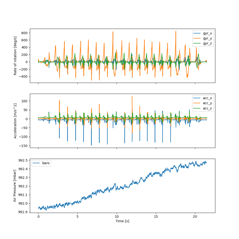
Below we plot all the relevant data for a single gait test to make it easier to understand.
For the selected test, we can see that the participant basically started walking right away. While it can not be easily seen from the raw data IMU itself, the participant walked down a stair in two bouts. This can be more clearly seen in the baro data, which shows a slowly increasing pressure value, indicating a reduction in altitude.
import matplotlib.pyplot as plt

foot = "right_sensor"
_, axs = plt.subplots(nrows=3, figsize=(10, 10), sharex=True)
imu_data[foot].filter(like="gyr").plot(ax=axs[0])
imu_data[foot].filter(like="acc").plot(ax=axs[1])
baro_data[foot].plot(ax=axs[2])

axs[0].set_ylabel("Rate of rotation [deg/s]")
axs[1].set_ylabel("Acceleration [m/s^2]")
axs[2].set_ylabel("Air Pressure [mbar]")
axs[2].set_xlabel("Time [s]")

plt.show()
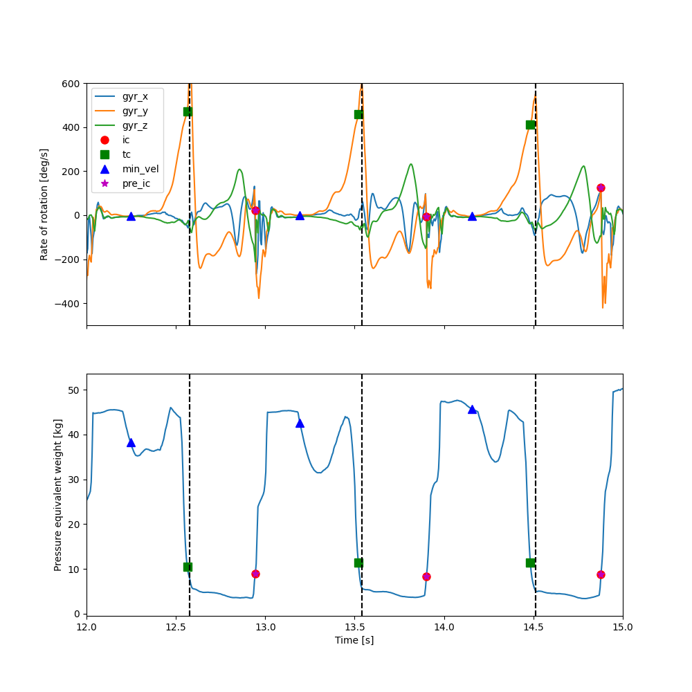
When zooming in we can see the individual events withing the strides.
The min_vel event is in the resting period between strides, and the IC and TC events at the falling and rising
edges of pressure signal, respectively.
The start and endpoints of the segmented strides (dashed lines) are at the maximum of the gyr_y signal.
foot = "right_sensor"
fig, axs = plt.subplots(nrows=2, figsize=(10, 10), sharex=True)
imu_data[foot].filter(like="gyr").plot(ax=axs[0])
pressure_data[foot]["total_force"].plot(ax=axs[1])
events = insole_events[foot].drop(columns=["start", "end"])
events /= datapoint.sampling_rate_hz
styles = ["ro", "gs", "b^", "m*"]
for style, (i, e) in zip(styles, events.T.iterrows()):
    e = e.dropna()
    axs[0].plot(e, imu_data[foot]["gyr_y"].loc[e.to_numpy()].to_numpy(), style, label=i, markersize=8)
    axs[1].plot(e, pressure_data[foot]["total_force"].loc[e.to_numpy()].to_numpy(), style, markersize=8)
for i, s in segmented_stride_list[foot].iterrows():
    s /= datapoint.sampling_rate_hz
    axs[0].axvline(s["start"], color="k", linestyle="--")
    axs[0].axvline(s["end"], color="k", linestyle="--")
    axs[1].axvline(s["start"], color="k", linestyle="--")
    axs[1].axvline(s["end"], color="k", linestyle="--")

axs[0].legend()
axs[0].set_xlim(12, 15)
axs[0].set_ylim(-500, 600)

axs[0].set_ylabel("Rate of rotation [deg/s]")
axs[1].set_ylabel("Pressure equivalent weight [kg]")
axs[1].set_xlabel("Time [s]")

plt.show()
StairAmbulationHealthy2021Full#
The StairAmbulationHealthy2021Full dataset is contains the complete recordings of all 20 participants, not cut into individual tests. Note, that there are still two recordings per participant. This is because data was collected at two different locations and hence, the data is split into two sections.
The StairAmbulationHealthy2021Full dataclass can be used equivalently to the StairAmbulationHealthyPerTest dataset. The only difference is that instead of the individual tests, we can see the two parts in the index for the dataset.
from gaitmap_datasets import StairAmbulationHealthy2021Full

dataset = StairAmbulationHealthy2021Full(
    include_pressure_data=True,
    include_baro_data=True,
    include_hip_sensor=True,
    memory=Memory("../.cache"),
)
dataset
subset = dataset.get_subset(participant="subject_01", part="part_2")
subset
As most parameters and attributes are identical, we will not repeat them.
One interesting addition is the test_list attribute.
If it is required to understand which tests where performed in the respective sessions, we can access them as a
region-of-interest list.
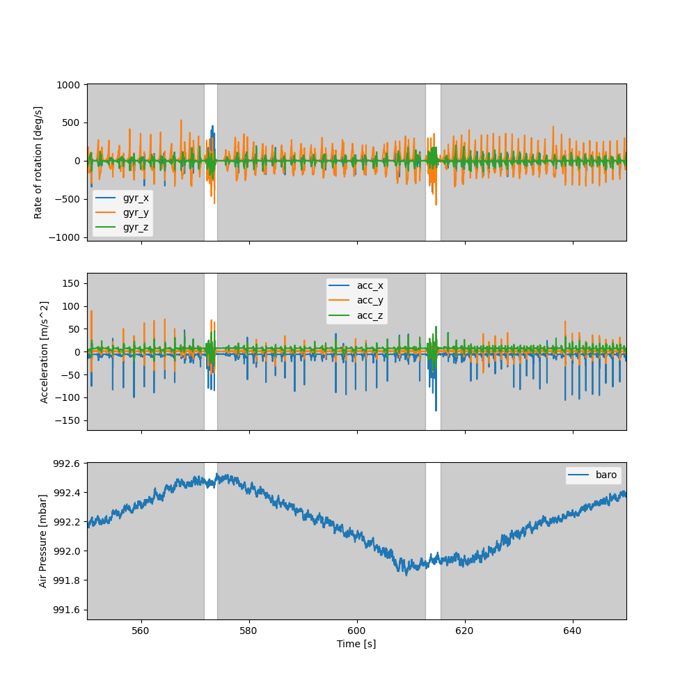
When plotting the data in the entire part_2 recording, we can see that it spans multiple tests including multiple
walks up and down various stairs.
If you would zoom in, you can see that between each test, the participants were instructed to jump up and down 3 times. These jump events were used as marker to cut the individual tests.
imu_data = subset.data
baro_data = subset.baro_data

foot = "right_sensor"
_, axs = plt.subplots(nrows=3, figsize=(10, 10), sharex=True)
imu_data[foot].filter(like="gyr").plot(ax=axs[0])
imu_data[foot].filter(like="acc").plot(ax=axs[1])
baro_data[foot].plot(ax=axs[2])
for i, s in subset.test_list.iterrows():
    s /= subset.sampling_rate_hz
    axs[0].axvspan(s["start"], s["end"], color="k", alpha=0.2)
    axs[1].axvspan(s["start"], s["end"], color="k", alpha=0.2)
    axs[2].axvspan(s["start"], s["end"], color="k", alpha=0.2)

axs[0].set_ylabel("Rate of rotation [deg/s]")
axs[1].set_ylabel("Acceleration [m/s^2]")
axs[2].set_ylabel("Air Pressure [mbar]")
axs[2].set_xlabel("Time [s]")

plt.xlim(550, 650)
plt.show()
A note on caching#
To make it possible to interact with the entire dataset, without filling your RAM immediately, all data is only
loaded once you access the respective data attribute (e.g. data or pressure_data).
However, this means, if you access the same piece of data multiple times (or multiple pieces of related data),
data needs to be loaded again from disk and preprocessed.
This is slow.
Therefore, we allow to use joblib.Memory to cache the data in a fast disk cache.
You can configure the cache directory using the memory parameter of the dataset class.
Keep in mind, that the cache directory can become quite large.
We recommend clearing the cache from time to time, to free up space.
Total running time of the script: ( 0 minutes 5.850 seconds)
Estimated memory usage: 142 MB