Kluge2017 - A dataset for in-lab parameter validation in healthy and PD.#

The Kluge 2017 dataset was recorded to test the validity of spatial-temporal parameters extracted from IMUs and their test-retest reliability. The dataset contains data from healthy participants and participants with Parkinson’s disease.

General information#

Each participant performed 4x10m walk trials at a slow, preferred and fast speed. Five of the participants performed the trials twice with two weeks in between.

The dataset contains IMU data from each foot recorded with the eGait system (sensor lateral attached to the shoe) and reference data using a marker-less Simi Motion system. Gait events were annotated manually based on the camera recordings und multiple points at the foot were tracked using the Simi Motion system.

For each 10m walk, only the middle 3 m are covered by the Simi Motion system, resulting on avaerage in 2-4 strides per walk-through.

The eGait system in the dataset used the Shimmer 3 sensors using a sampling rate of 102.4 Hz. For the data loaded using the dataset class, we adjust the coordinate system as shown in the figure below. While the sensor configuration is identical to other Shimmer 3 datasets, the coordiante system of the exported data was already rotated to align both feets. Hence, we need to perform a different coordinate transformation than for the other datasets:

coordinate system definition

Warning

For this example to work, you need to have a global config set containing the path to the dataset. Check the README.md for more information.

from gaitmap_datasets import Kluge2017

First we will create a simple instance of the dataset class. We can see that for each participant we have 3 different walking speeds, the information if they are healthy or PD (patient = True) and if the data was recorded in the first or second session.

dataset = Kluge2017()
dataset

Kluge2017 [75 groups/rows]

patient participant repetition speed
0 False 216060 0 fast
1 False 216060 0 normal
2 False 216060 0 slow
3 False 216061 1 fast
4 False 216061 1 normal
... ... ... ... ...
70 True 215001 0 normal
71 True 215001 0 slow
72 True 413050 0 fast
73 True 413050 0 normal
74 True 413050 0 slow

75 rows × 4 columns


Based on the index, we will select just the PD cohort

pd_cohort = dataset.get_subset(patient=True)
pd_cohort

Kluge2017 [12 groups/rows]

patient participant repetition speed
0 True 115053 0 fast
1 True 115053 0 normal
2 True 115053 0 slow
3 True 214019 0 fast
4 True 214019 0 normal
5 True 214019 0 slow
6 True 215001 0 fast
7 True 215001 0 normal
8 True 215001 0 slow
9 True 413050 0 fast
10 True 413050 0 normal
11 True 413050 0 slow


We will simply select the first participant in the dataset for the following analysis

participant = pd_cohort.groupby("participant")[0].groupby(None)
participant

Kluge2017 [3 groups/rows]

patient participant repetition speed
0 True 115053 0 fast
1 True 115053 0 normal
2 True 115053 0 slow


Let’s have a look at the slow walk data

slow_walk = participant.get_subset(speed="slow")
slow_walk

Kluge2017 [1 groups/rows]

patient participant repetition speed
0 True 115053 0 slow


For each gait test, we have access to the raw IMU data, the marker position data and the gait events. Let’s have a look at the raw IMU data. This is a dictionary with the sensor name as key and a pandas DataFrame as value. Note that the index is the time in seconds already aligned with the mocap data.

foot = "right"

imu_data = slow_walk.data[f"{foot}_sensor"]
imu_data
acc_x acc_y acc_z gyr_x gyr_y gyr_z
time after start [s]
0.007812 -0.606944 -0.806221 9.749680 -0.233754 -2.983602 1.094100
0.017578 -0.529068 -0.844837 9.633973 0.691206 -3.561525 0.420545
0.027344 -0.490796 -0.768402 9.555994 0.989510 -4.397582 0.238766
0.037109 -0.452116 -0.768090 9.556089 2.782382 -4.679503 0.113708
0.046875 -0.490779 -0.843053 9.827733 4.531894 -4.103905 -0.197483
... ... ... ... ... ... ...
65.544922 -0.721370 -1.037000 9.789950 0.419637 11.173907 3.775545
65.554688 -0.837001 -1.114059 9.867739 3.130379 12.023181 4.900520
65.564453 -0.953323 -1.076638 9.867153 3.852850 12.442962 5.295863
65.574219 -0.952116 -1.230358 9.829633 4.541235 12.803124 5.783288
65.583984 -0.991486 -1.116189 9.751162 5.986108 12.502267 6.087537

6716 rows × 6 columns


Then let’s also load the marker position data. As all markers trajectories have the same length, this is just a simple pandas DataFrame, with the foot as the top-most column level. We can see that we get position, velocity and acceleration data for the ankle and the tip of the foot. Note that these trajectories are from “actual” markers, but virtual markers defined by the biomechanical model fitted by the SIMI system.

Many values in the dataframe will be NaN, as the mocap system only tracks the foot for a short period of time.

mocap_data = slow_walk.marker_position_[foot]
mocap_data
marker ankle foot_tip
metric pos_x pos_y pos_z vel_x vel_y vel_z acc_x acc_y acc_z pos_x pos_y pos_z vel_x vel_y vel_z acc_x acc_y acc_z
time after start [s]
1.000000e-06 NaN NaN NaN NaN NaN NaN NaN NaN NaN NaN NaN NaN NaN NaN NaN NaN NaN NaN
9.995000e-03 NaN NaN NaN NaN NaN NaN NaN NaN NaN NaN NaN NaN NaN NaN NaN NaN NaN NaN
1.999800e-02 NaN NaN NaN NaN NaN NaN NaN NaN NaN NaN NaN NaN NaN NaN NaN NaN NaN NaN
3.000000e-02 NaN NaN NaN NaN NaN NaN NaN NaN NaN NaN NaN NaN NaN NaN NaN NaN NaN NaN
3.999400e-02 NaN NaN NaN NaN NaN NaN NaN NaN NaN NaN NaN NaN NaN NaN NaN NaN NaN NaN
... ... ... ... ... ... ... ... ... ... ... ... ... ... ... ... ... ... ...
6.555000e+01 NaN NaN NaN NaN NaN NaN NaN NaN NaN NaN NaN NaN NaN NaN NaN NaN NaN NaN
6.555999e+01 NaN NaN NaN NaN NaN NaN NaN NaN NaN NaN NaN NaN NaN NaN NaN NaN NaN NaN
6.557000e+01 NaN NaN NaN NaN NaN NaN NaN NaN NaN NaN NaN NaN NaN NaN NaN NaN NaN NaN
6.557999e+01 NaN NaN NaN NaN NaN NaN NaN NaN NaN NaN NaN NaN NaN NaN NaN NaN NaN NaN
6.558999e+01 NaN NaN NaN NaN NaN NaN NaN NaN NaN NaN NaN NaN NaN NaN NaN NaN NaN NaN

6560 rows × 18 columns


Let’s plot the position of the foot marker and the IMU data together.

import matplotlib.pyplot as plt

fig, (ax1, ax2, ax3, ax4, ax5) = plt.subplots(nrows=5, sharex=True, figsize=(10, 10))
fig.suptitle(f"{slow_walk.group} - {foot} foot")
# Plot the IMU data
ax1.set_title("Gyro")
ax1.set_ylabel("deg/s")
imu_data.filter(like="gyr").plot(ax=ax1)
ax2.set_title("Acc")
ax2.set_ylabel("m/s²")
imu_data.filter(like="acc").plot(ax=ax2)

# Plot the mocap data
ax3.set_title("Marker position X")
ax3.set_ylabel("m")
mocap_data.xs("pos_x", level=1, axis=1).plot(ax=ax3)
ax4.set_title("Marker position Y")
ax4.set_ylabel("m")
mocap_data.xs("pos_y", level=1, axis=1).plot(ax=ax4)
ax5.set_title("Marker position Z")
ax5.set_ylabel("m")
mocap_data.xs("pos_z", level=1, axis=1).plot(ax=ax5)

plt.tight_layout()
plt.show()
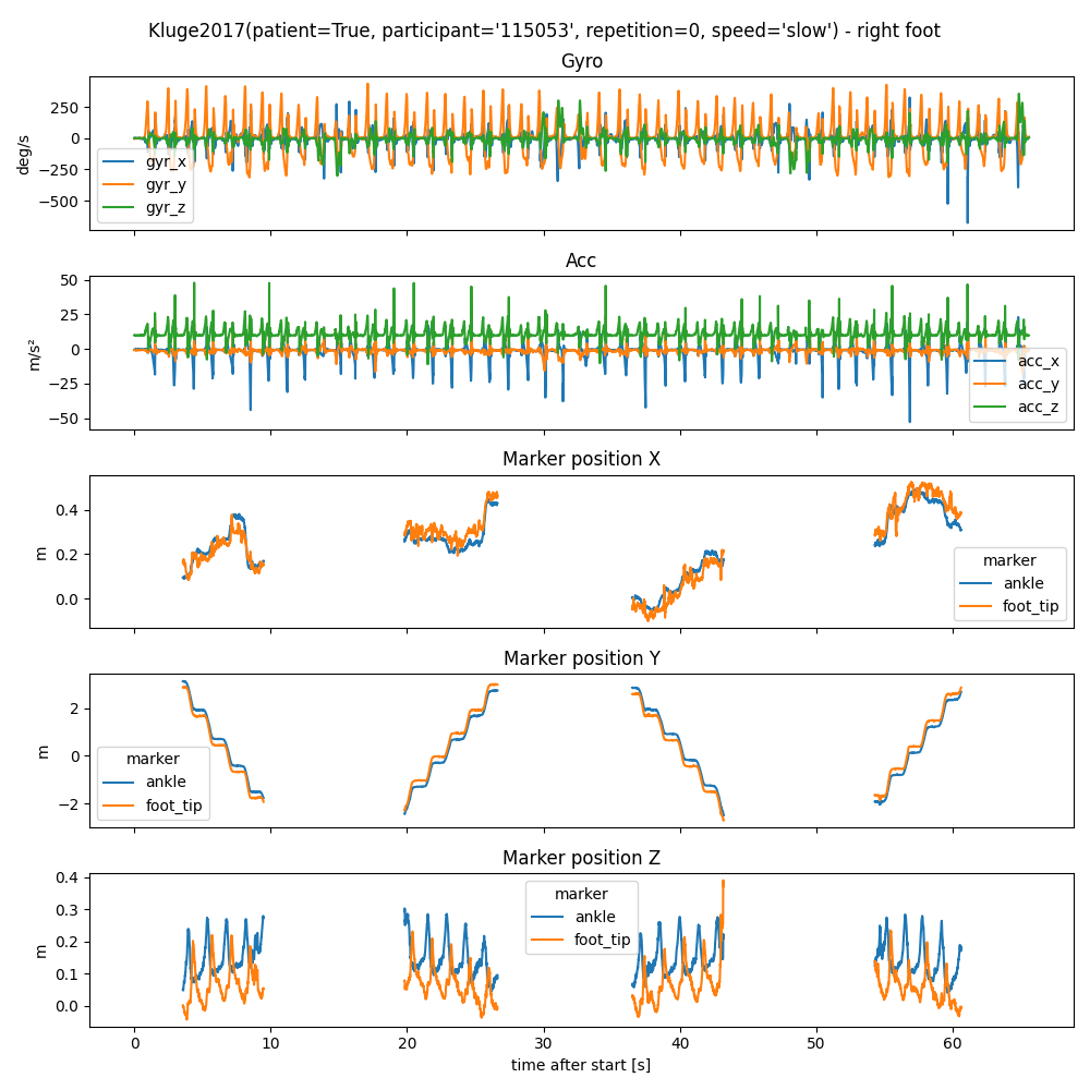
Kluge2017(patient=True, participant='115053', repetition=0, speed='slow') - right foot, Gyro, Acc, Marker position X, Marker position Y, Marker position Z

We can also plot the gait events on top of the data. The gait events are stored in a dictionary with the foot as key and a pandas DataFrame as value. Each row in the DataFrame represents one gait stride. Each stride starts and ends with a heel strike/initial contact (IC) of the same foot. The HS event provided with the stride is the start event. In addition, we have the toe-off (TO), the heel-off (HO). The terminal contact (TC) is either the TO or the HO depending on which event occurs last.

All events are provided as samples in the Mocap data.

gait_events = slow_walk.mocap_events_[foot]
gait_events
event ho ic to start end tc
s_id
54 508 438 527 438 576 527
56 650 576 669 576 722 669
58 788 722 811 722 854 811
67 2121 2047 2146 2047 2196 2146
69 2256 2196 2279 2196 2330 2279
71 2402 2330 2418 2330 2467 2418
73 2532 2467 2558 2467 2607 2558
84 3813 3749 3841 3749 3892 3841
86 3964 3892 3986 3892 4037 3986
88 4105 4037 4129 4037 4182 4129
90 4241 4182 4265 4182 4314 4265
97 5618 5553 5644 5553 5681 5644
99 5737 5681 5766 5681 5820 5766
101 5884 5820 5910 5820 5961 5910


Let’s plot the gait events on top of the data.

import matplotlib.pyplot as plt


def plot_with_marker():
    fig, (ax1, ax2, ax3) = plt.subplots(nrows=3, sharex=True, figsize=(10, 6))
    fig.suptitle(f"{slow_walk.group} - {foot} foot")

    # Plot the IMU data
    ax1.set_title("Gyro")
    ax1.set_ylabel("deg/s")
    imu_data.filter(like="gyr").plot(ax=ax1)
    ax2.set_title("Acc")
    ax2.set_ylabel("m/s²")
    imu_data.filter(like="acc").plot(ax=ax2)

    # Plot the mocap data
    ax3.set_title("Marker position ankle Z")
    ax3.set_ylabel("m")
    mocap_data[("ankle", "pos_z")].plot(ax=ax3)

    # Plot the gait events
    for i, (_, stride_mocap) in enumerate(gait_events.iterrows()):
        stride_time = stride_mocap / slow_walk.mocap_sampling_rate_hz_
        stride_imu = (stride_time * slow_walk.sampling_rate_hz).round().astype(int)

        for ax, plot_data in zip(
            (ax1, ax2, ax3), (imu_data["gyr_y"], imu_data["acc_x"], mocap_data[("ankle", "pos_z")])
        ):
            # Plot the stride as a vertical span
            ax.axvspan(stride_time.start, stride_time.end, alpha=0.2, edgecolor="black")

            index_values = stride_imu
            if ax == ax3:
                index_values = stride_mocap

            # Plot the individual events
            ax.plot(stride_time.to, plot_data.iloc[index_values.to], "s", color="blue", label="to" if i == 0 else None)
            ax.plot(stride_time.ho, plot_data.iloc[index_values.ho], "o", color="red", label="ho" if i == 0 else None)
            ax.plot(stride_time.tc, plot_data.iloc[index_values.tc], "x", color="green", label="tc" if i == 0 else None)

    ax3.legend()

    return fig, (ax1, ax2, ax3)


plot_with_marker()
plt.tight_layout()
plt.show()
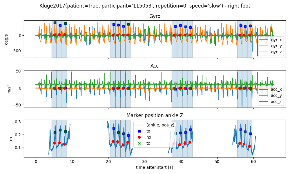
Kluge2017(patient=True, participant='115053', repetition=0, speed='slow') - right foot, Gyro, Acc, Marker position ankle Z

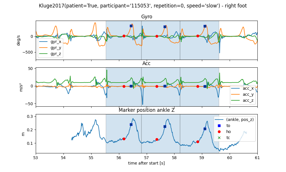
To better see what is going on, we will zoom into one WB.
_, (_, _, ax3) = plot_with_marker()
ax3.set_xlim(53, 61)
plt.show()
Kluge2017(patient=True, participant='115053', repetition=0, speed='slow') - right foot, Gyro, Acc, Marker position ankle Z

We can see that all the gait events occur in order and roughly line up with the expected signal regions in the IMU signal. We can also see that the z-axis of the ankle marker is drifting over the course of each walk. This is because the mocap system is not calibrated level to the floor. In case parameters like foot-clearance are calculated, this needs to be taken into account.

Spatial Parameters#

In case you want to caluclate spatial parameters based on the trajectories and events, you can use the marker_position_per_stride_ property. It provides the marker information per stride, making it easy to calculate various parameters

per_stride = slow_walk.marker_position_per_stride_[foot]
per_stride
marker ankle foot_tip
metric pos_x pos_y pos_z vel_x vel_y vel_z acc_x acc_y acc_z pos_x pos_y pos_z vel_x vel_y vel_z acc_x acc_y acc_z
s_id sample
54 0 0.192753 1.958257 0.082491 0.286104 -0.200563 -0.097244 0.721611 8.414624 0.803715 0.200133 1.704741 0.176551 0.080548 -0.418227 -0.721726 -13.600050 5.803189 -11.501573
1 0.193070 1.950421 0.071967 0.261980 -0.049779 -0.071751 0.374040 9.592503 8.698684 0.201110 1.698432 0.169994 -0.039450 -0.267904 -0.710838 -12.476939 7.288913 -3.356514
2 0.199773 1.955140 0.077238 0.248103 -0.058738 -0.091036 -4.638317 8.426217 8.246024 0.193884 1.695691 0.153551 -0.339818 -0.270176 -0.831751 -5.776758 8.854914 4.857469
3 0.203452 1.954273 0.079510 0.274201 -0.068357 0.102675 -6.699009 -0.698306 3.084113 0.190630 1.694360 0.153355 -0.479444 -0.299115 -0.793489 -2.950642 1.387353 4.389224
4 0.203464 1.954910 0.077449 0.112368 0.150302 0.275149 -6.473012 -5.153564 1.867230 0.189794 1.693608 0.146054 -0.278234 -0.048348 -0.523989 1.823821 -3.238908 3.602642
... ... ... ... ... ... ... ... ... ... ... ... ... ... ... ... ... ... ... ...
101 137 0.349034 2.297499 0.056475 -0.493256 0.644704 -0.112424 1.574143 -5.545146 -4.041856 0.410542 2.556118 0.106533 0.308624 0.591946 -0.671209 -8.179141 -3.797458 -10.331998
138 0.349848 2.298396 0.057959 -0.397720 0.497977 -0.291812 -1.411988 -3.820587 -4.530557 0.417965 2.557068 0.098224 0.125974 0.469589 -0.713592 -3.917129 -3.669168 -10.004805
139 0.344574 2.310484 0.058835 -0.205808 0.457452 -0.254028 5.376377 -6.819976 -5.684798 0.410538 2.570010 0.097141 -0.075496 0.476007 -0.643591 -7.225660 -5.294753 -3.979611
140 0.339505 2.324432 0.051485 -0.363760 0.522266 -0.151031 10.019334 -7.228755 1.519903 0.418452 2.579842 0.092782 0.004334 0.487045 -0.719070 -11.001638 -3.606945 3.266294
141 0.340955 2.317538 0.045446 -0.296046 0.402155 -0.327242 5.374675 -6.203757 8.011034 0.408858 2.577185 0.079282 -0.026589 0.370898 -0.776057 -5.104494 -4.194661 4.593462

1963 rows × 18 columns


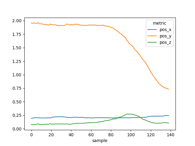
To extract the information of a single stride (e.g. stride_ist 55), we can use the loc method.

marker ankle foot_tip
metric pos_x pos_y pos_z vel_x vel_y vel_z acc_x acc_y acc_z pos_x pos_y pos_z vel_x vel_y vel_z acc_x acc_y acc_z
sample
0 0.192753 1.958257 0.082491 0.286104 -0.200563 -0.097244 0.721611 8.414624 0.803715 0.200133 1.704741 0.176551 0.080548 -0.418227 -0.721726 -13.600050 5.803189 -11.501573
1 0.193070 1.950421 0.071967 0.261980 -0.049779 -0.071751 0.374040 9.592503 8.698684 0.201110 1.698432 0.169994 -0.039450 -0.267904 -0.710838 -12.476939 7.288913 -3.356514
2 0.199773 1.955140 0.077238 0.248103 -0.058738 -0.091036 -4.638317 8.426217 8.246024 0.193884 1.695691 0.153551 -0.339818 -0.270176 -0.831751 -5.776758 8.854914 4.857469
3 0.203452 1.954273 0.079510 0.274201 -0.068357 0.102675 -6.699009 -0.698306 3.084113 0.190630 1.694360 0.153355 -0.479444 -0.299115 -0.793489 -2.950642 1.387353 4.389224
4 0.203464 1.954910 0.077449 0.112368 0.150302 0.275149 -6.473012 -5.153564 1.867230 0.189794 1.693608 0.146054 -0.278234 -0.048348 -0.523989 1.823821 -3.238908 3.602642
... ... ... ... ... ... ... ... ... ... ... ... ... ... ... ... ... ... ...
134 0.241468 0.760751 0.111336 0.218162 -0.831061 -0.031026 2.153917 12.167150 -7.792384 0.228153 0.509273 0.210098 -0.539473 -0.926413 -0.252263 0.766407 8.995751 -18.505880
135 0.244614 0.751074 0.111428 0.156707 -0.754187 -0.101599 0.823188 17.730366 -7.090275 0.218403 0.501140 0.211520 -0.561376 -0.832486 -0.322680 7.949738 13.164203 -22.556181
136 0.243416 0.744900 0.107063 0.244162 -0.764780 -0.175111 0.471186 14.072620 -4.902506 0.232609 0.492156 0.202855 -0.305319 -0.796774 -0.360671 4.651704 12.463881 -15.043660
137 0.244126 0.741234 0.109109 0.306830 -0.430380 -0.218322 4.352034 8.988792 -4.125971 0.221726 0.487249 0.199454 -0.072033 -0.549494 -0.702970 2.152110 10.498327 -9.447768
138 0.243791 0.727777 0.106066 0.235850 -0.244594 -0.201803 4.433455 11.586198 -1.939656 0.223650 0.473770 0.196879 -0.239267 -0.394179 -0.823661 -2.620951 12.868330 -10.005720

139 rows × 18 columns


fig, ax = plt.subplots()
stride_54["ankle"].filter(like="pos_").plot(ax=ax)

fig.show()
kluge 2017

Further Notes#

  1. When applying a train test split on the data, remember that some participants have multiple recordings. Hence, always group by participant before splitting (see tpcp documentation for more details).

  2. When comparing the results of an IMU algorithm to the mocap data, the recommended way is to compare based on aggregated values over the entire gait test, as alignment of individual strides might not always be possible and hide issues, when an algorithm is missing multiple strides. However, keep in mind that the mocap system only covers the middle part of each walk. This means that when comparing aggregated values (in particular measures of variance) using all detected strides in the IMU signal might result in a biased comparison.

  3. When calculating spatial parameters, we recommend the use of the ankle trajectory, as it is the most stable trajectory.

Total running time of the script: ( 0 minutes 24.243 seconds)

Estimated memory usage: 682 MB

Gallery generated by Sphinx-Gallery