Note
Click here to download the full example code
EgaitAdidas2014 - Healthy Participants with MoCap reference#
This dataset contains data from healthy participants walking with different speed levels through a motion capture volume. The dataset can be used to benchmark the performance of spatial parameter estimation methods based on foot worn IMUs.
General Information#
The EgaitAdidas2014 dataset contains data healthy participants walking through a vicon motion capture system with one IMU attached to each foot.
For many participants data for SHIMMER3 and SHIMMER2 is available. The SHIMMER3 data is sampled at 204.8 Hz and the SHIMMER2R data at 102.4 Hz. This also allows for a comparison of the two sensors.
For both IMUs we unify the coordinate system on loading as shown below:


Participants where instructed to walk with a specific stride length and velocity to create more variation in the data. For each trial only a couple strides were recorded within the motion capture system. The IMU data contains the entire recording. This additional data can contain just some additional strides or entire different movements depending on the trial. We recommend inspecting the specific trial in case of issues.
The Vicon motion capture system was sampled at 200 Hz. The IMUs and the mocap system are synchronized using a wireless trigger allowing for proper comparison of the calculated trajectories.
Reference (expert labeled based on IMU data) stride borders are provided for all strides that are recorded by both systems.
In the following we will show how to interact with the dataset and how to make sense of the reference information.
Warning
For this example to work, you need to have a global config set containing the path to the dataset.
Check the README.md for more information.
First we create a simple instance of the dataset class.
from gaitmap_datasets import EgaitAdidas2014
from gaitmap_datasets.utils import convert_segmented_stride_list

dataset = EgaitAdidas2014()
dataset
We can see that we have 5 levels in the metadata.
participant
sensortype (shimmer2, shimmer3)
stride_length (low, medium, high)
stride_velocity (low, medium, high)
repetition (1, 2, 3)
The stride_length and stride_velocity are the instructions given to the participants.
For each combination of these two parameters, 3 repetitions were recorded.
However, for many participants data for at least some trials are missing for various technical issues.
For now we are selecting the data for one participant.
subset = dataset.get_subset(participant="008")
subset
For this participant we will have a look at the “normal” stride length and velocity trial of the shimmer2r sensor.
trial = subset.get_subset(stride_length="normal", stride_velocity="normal", sensor="shimmer2r", repetition="1")
trial
The IMU data is stored in the data attribute, which is a dictionary of pandas dataframes.
The mocap data is stored in the marker_position_ attribute, which is a dictionary of pandas dataframes, too.
Note, that sometimes there are NaN values at the start and the end of the data.
In these regions the mocap system was recording, but none of the markers were in frame.
mocap_data = trial.marker_position_[sensor]
mocap_data
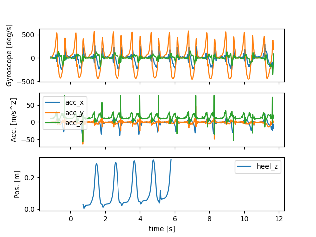
Both data sources have the time as index, so that we can easily plot them together. We converted the time axis so that the start of the Mocap data is the global 0. This means that the IMU data will have negative time values for the datapoints before the MoCap start.
import matplotlib.pyplot as plt

fig, (ax1, ax2, ax3) = plt.subplots(3, 1, sharex=True)
imu_data.filter(like="gyr").plot(ax=ax1, legend=False)
imu_data.filter(like="acc").plot(ax=ax2, legend=True)
mocap_data[["heel_z"]].plot(ax=ax3)

ax1.set_ylabel("Gyroscope [deg/s]")
ax2.set_ylabel("Acc. [m/s^2]")
ax3.set_ylabel("Pos. [m]")

fig.show()
For the strides that are within the mocap volume, manually annotated stride labels based on the IMU data are available. They are provided in samples relative to the start of the IMU data stream.
segmented_strides = trial.segmented_stride_list_
segmented_strides[sensor]
To get the events relative to the mocap data (i.e. in mocap samples relative to the start of the mocap data you can
use the convert_events method.
trial.convert_events(segmented_strides, from_time_axis="imu", to_time_axis="mocap")[sensor]
Similarly, you can convert the events to the same time axis as the data
trial.convert_events(segmented_strides, from_time_axis="imu", to_time_axis="time")[sensor]
In addition to the segmented strides, we also provide a reference event list calculated based on the mocap data. This has the same start and end per stride as the segmented strides, but has columns for the initial contact/heel strike (ic), final contact/toe off (tc) and mid-stance (min_vel). This information is provided in samples relative to the start of the mocap data stream. (Compare to the converted segmented strides above).
mocap_events = trial.mocap_events_
mocap_events[sensor]
Like the segmented stride list, we can convert them to the same time axis as the data or IMU samples.
trial.convert_events(mocap_events, from_time_axis="mocap", to_time_axis="time")[sensor]
Below we plot the time converted event list into the plot from above In the mocap plot we also add the mocap derived gait events.
fig, (ax1, ax2, ax3) = plt.subplots(3, 1, sharex=True)
imu_data.filter(like="gyr").plot(ax=ax1, legend=False)
imu_data.filter(like="acc").plot(ax=ax2, legend=True)
mocap_data[["heel_z"]].plot(ax=ax3)
for ax in (ax1, ax2, ax3):
    for i, s in trial.convert_events(segmented_strides, from_time_axis="imu", to_time_axis="time")[sensor].iterrows():
        ax.axvspan(s["start"], s["end"], alpha=0.2, color="C1")

# We plot the events in ax3
for marker, event_name in zip(["o", "s", "*"], ["tc", "ic", "min_vel"]):
    mocap_data[["heel_z"]].iloc[mocap_events[sensor][event_name]].rename(columns={"heel_z": event_name}).plot(
        ax=ax3, style=marker, label=event_name, markersize=3
    )

ax1.set_ylabel("Gyroscope [deg/s]")
ax2.set_ylabel("Acc. [m/s^2]")
ax3.set_ylabel("Pos. [m]")

fig.show()
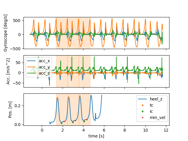
As you can see, in this example, three strides are properly detected by both systems.
These strides are defined based on the signal maximum in the gyr_y (i.e. gyr_ml axis).
This definition is good for segmentation.
However, for calculation of gait parameters, the authors of the dataset defined strides from midstance (i.e. the
min_vel point) to midstance of two consecutive strides.
In result, when looking at the parameters, there will be one stride less than the number of strides in the segmented
stride list.
trial.mocap_parameters_[sensor]
To better understand how this works, we can convert the mocap events from their segmented stride list form into a
min_vel-stride list.
In this form, the start and the end of each stride is defined by the min_vel event.
In addition, a new pre_ic event is added.
This marks the ic of the previous stride.
Overall, one less stride exists in the min_vel stride list than in the segmented stride list.
The s_id of the new stride list is based on the s_id of the segmented stride that contains the pre_ic event.
mocap_min_vel_stride_list = convert_segmented_stride_list(mocap_events, target_stride_type="min_vel")
mocap_min_vel_stride_list[sensor]
Stride time is now calculated from the pre_ic to the ic event (compare trial.mocap_parameters_[sensor]).
stride_time = mocap_min_vel_stride_list[sensor]["ic"] - mocap_min_vel_stride_list[sensor]["pre_ic"]
stride_time / trial.mocap_sampling_rate_hz_
s_id
0    1.085
1    1.085
dtype: float64
As comparison the pre-calculated stride time:
trial.mocap_parameters_[sensor]["stride_time"]
s_id
0    1.085
1    1.085
Name: stride_time, dtype: float64
Stride length is calculated as the displacement in the ground-plane between start and end (i.e. the two min_vel
events).
starts = mocap_min_vel_stride_list[sensor]["start"]
ends = mocap_min_vel_stride_list[sensor]["end"]
stride_length_heel = (
    (
        mocap_data[["heel_x", "heel_y"]].iloc[ends].reset_index(drop=True)
        - mocap_data[["heel_x", "heel_y"]].iloc[starts].reset_index(drop=True)
    )
    .pow(2)
    .sum(axis=1)
    .pow(0.5)
)
stride_length_heel
0    1.478275
1    1.474500
dtype: float32
As comparison the pre-calculated stride length: Note that this stride-length differs slightly from the one calculated above, as the authors of the dataset provided the average stride length over all available markers.
trial.mocap_parameters_[sensor]["stride_length"]
s_id
0    1.479162
1    1.474048
Name: stride_length, dtype: float64
Usage as validation dataset#
To compare the reference parameters with the parameters of a IMU based algorithm, you should use the segmented
stride list as a starting point.
From there you can calculate gait events (e.g. ic) within these strides to compare temporal parameters.
Ideally store the events as a segmented stride list and then use the convert_segmented_stride_list function to
bring them in the same format used to calculate the reference parameters.
When calculating spatial parameters, you should calculate your own IMU based min_vel points instead of using the mocap derived ones. These don’t always align with real moments of no movement in the IMU data and hence might lead to issues with ZUPT based algorithms.
For algorithms that rely on calculations on the entire signal (i.e. not just the strides within the mocap volume), keep in mind, that the amount of additional movement in the data varies from trial to trial. Some trials just contain walking, others resting and walking, and some contain small jumps used as fallback synchronization. Hence, if you see unexpected results for specific trails, you might want to check the raw data.
Further Notes#
In many cases clear drift in the Mocap data is observed. The authors of the dataset corrected that drift before calculating the reference parameters using a linear drift model. For further information see the two papers using the dataset [1] and [2].
Total running time of the script: ( 0 minutes 5.632 seconds)
Estimated memory usage: 24 MB