Note
Click here to download the full example code
SensorPositionComparison2019 - Full mocap reference data set with 6 sensors per foot#
We provide 2 versions of the dataset:
- SensorPositionComparison2019Segmentation:
In this dataset no Mocap ground truth is provided and the IMU data is not cut to the individual gait test, but just a single recording for all participants exists with all tests (including failed ones) and movement between the tests. This can be used for stride segmentation tasks, as we hand-labeled all stride-start-end events in these recordings
- SensorPositionComparison2019Mocap:
In this dataset the data is cut into the individual tests. This means 7 data segments exist per participants. For each of these segments full synchronised motion capture reference is provided.
For more information about the dataset, see the dataset [documentation](https://zenodo.org/record/5747173)
General information#
The dataset was recorded with Nilspod sensors by Portabiles. Multiple sensors were attached to the feet of the participants. For most tasks you will only be interested in the data from one sensor position.
The data from all foot-mounted IMUs are transformed into the gaitmap coordinate system on loading. If you want to use the data from the ankle or hip sensor, they will remain in their original coordinate system as defined by the sensor node. For attachment images see the dataset [documentation](https://zenodo.org/record/5747173).
Below we show the performed dataset transformation for the instep sensor as an example. All other sensor transformations are shown at the end of this document.

Warning
For this example to work, you need to have a global config set containing the path to the dataset.
Check the README.md for more information.
SensorPositionComparison2019Segmentation#
This version of the dataset contains one recording per participant with all tests and movement between the tests. No Mocap reference is provided, but just the IMU data and the stride borders based on the IMU data.
By default, the data of all sensors is provided and the data for each sensor is aligned based on the roughly known orientation of the sensor, so that the coordinate system of the insole sensor (see dataset documentation) can be used for all sensors.
from joblib import Memory

from gaitmap_datasets.sensor_position_comparison_2019 import SensorPositionComparison2019Segmentation

dataset = SensorPositionComparison2019Segmentation(
    memory=Memory("../.cache"),
)
dataset
We can see that we have 14 participants. Using the dataset class, we can select any subset of participants.
subset = dataset.get_subset(participant=["4d91", "5047"])
subset
Once we have the selection of data we want to work with, we can iterate the dataset object to access the data of individual datapoints or just index it as below.
datapoint = subset[0]
datapoint
On this datapoint, we can now access the data. We will start with the metadata.
datapoint.metadata
{'age': 28.0, 'bmi': 24.69, 'height': 180.0, 'imu_tests': {'fast_10': {'start': '2019-05-29T11:56:00.131836000', 'start_idx': 37914, 'stop': '2019-05-29T11:56:29.545898000', 'stop_idx': 43938}, 'fast_20': {'start': '2019-05-29T11:59:27.661132000', 'start_idx': 80416, 'stop': '2019-05-29T11:59:55.737304000', 'stop_idx': 86166}, 'long': {'start': '2019-05-29T12:00:19.760742000', 'start_idx': 91086, 'stop': '2019-05-29T12:05:26.264648000', 'stop_idx': 153858}, 'normal_10': {'start': '2019-05-29T11:53:28.408203000', 'start_idx': 6841, 'stop': '2019-05-29T11:54:12.934570000', 'stop_idx': 15960}, 'normal_20': {'start': '2019-05-29T11:57:03.544922000', 'start_idx': 50901, 'stop': '2019-05-29T11:57:38.671875000', 'stop_idx': 58095}, 'slow_10': {'start': '2019-05-29T11:54:38.159179000', 'start_idx': 21126, 'stop': '2019-05-29T11:55:34.155273000', 'stop_idx': 32594}, 'slow_20': {'start': '2019-05-29T11:58:09.355468000', 'start_idx': 64379, 'stop': '2019-05-29T11:59:03.520507000', 'stop_idx': 75472}}, 'mocap_test_start': {'fast_10': '2019-05-29, 13:55:57', 'fast_20': '2019-05-29, 13:59:24', 'long': '2019-05-29, 14:00:16', 'normal_10': '2019-05-29, 13:53:25', 'normal_20': '2019-05-29, 13:57:00', 'slow_10': '2019-05-29, 13:54:35', 'slow_20': '2019-05-29, 13:58:06'}, 'sensors': {'back': 'A515', 'l_ankle': 'E901', 'l_cavity': '9CA5', 'l_heel': '598E', 'l_insole': 'EFCC', 'l_instep': 'D60A', 'l_lateral': 'EB9E', 'l_medial': '5D89', 'r_ankle': 'C9FB', 'r_cavity': '9710', 'r_heel': '36BD', 'r_insole': '6807', 'r_instep': '922A', 'r_lateral': '0D14', 'r_medial': '220F', 'sync': '323C'}, 'sex': 'male', 'shoe_size': 42, 'weight': 80.0}
Next we can access the synchronised data of the individual sensors. The data is stored as a multi-column pandas DataFrame with the time as index.
imu_data = datapoint.data
imu_data.head()
________________________________________________________________________________
[Memory] Calling gaitmap_datasets.sensor_position_comparison_2019._dataset._get_session_and_align...
_get_session_and_align('4d91', data_folder=PosixPath('/home/arne/Documents/repos/work/projects/sensor_position_comparison/sensor_position_main_analysis/data/raw'))
____________________________________________get_session_and_align - 5.3s, 0.1min
Finally, we provide hand-labeled stride borders for the IMU data. All strides are labeled based on the minima in the gyr_ml signal (see dataset documentation for more details).
Note that we use a trailing _ to indicate that this is data calculated based on the ground truth/manual labels and
not just the IMU data.
segmented_stride_labels = datapoint.segmented_stride_list_["left"]
segmented_stride_labels.head()
Alternatively to the segmented_stride_list_ we also provide the segmented_stride_list_per_sensor_ makes it
easier to directly access the stride borders for a specific sensor (note they are still the same, as before,
as only one stridelist per foot exists).
segmented_stride_labels = datapoint.segmented_stride_list_per_sensor_["l_insole"]
segmented_stride_labels.head()
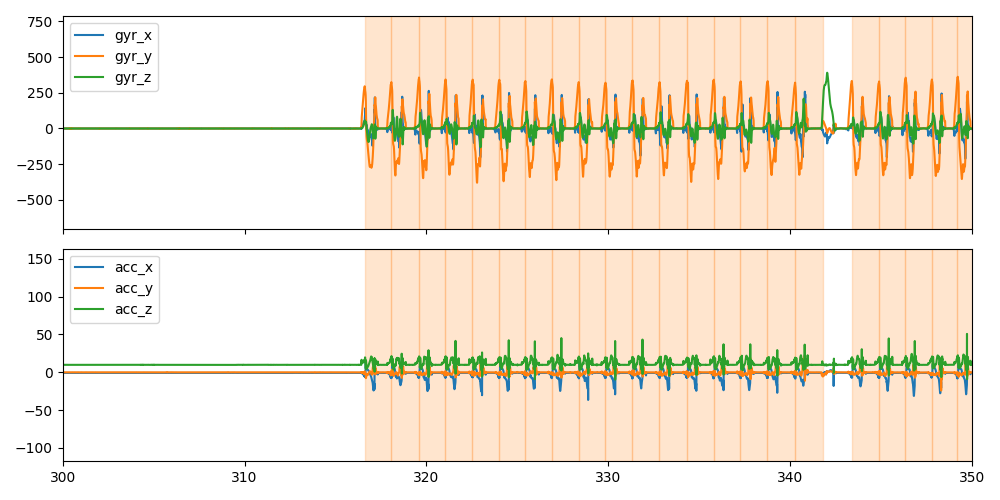
Below we plot the IMU data (acc on top, gyro on bottom) and the stride borders for a small part of the data.
import matplotlib.pyplot as plt

sensor = "l_insole"
fig, axes = plt.subplots(2, 1, sharex=True, figsize=(10, 5))
imu_data[sensor].filter(like="gyr").plot(ax=axes[0])
imu_data[sensor].filter(like="acc").plot(ax=axes[1])
for i, s in datapoint.segmented_stride_list_["left"].iterrows():
    s /= datapoint.sampling_rate_hz
    axes[0].axvspan(s["start"], s["end"], alpha=0.2, color="C1")
    axes[1].axvspan(s["start"], s["end"], alpha=0.2, color="C1")

axes[0].set_xlim(300, 350)
fig.tight_layout()
fig.show()
SensorPositionComparison2019Mocap#
For this version of the dataset, the data is split into the individual tests. This means 7 data segments exist per participants. For details about the respective tests, see the dataset documentation.
For each of these segments full synchronised motion capture trajectory of all markers is provided. Further, we provide labels for IC and TC derived from the motion capture data for each of the hand labeled strides within the segments.
from gaitmap_datasets.sensor_position_comparison_2019 import SensorPositionComparison2019Mocap

dataset = SensorPositionComparison2019Mocap(
    memory=Memory("../.cache"),
)
dataset
We can see that one individual data point for this dataset is only one of the gaittests.
datapoint = dataset[0]
datapoint
We can access the entire trajectory of the motion capture markers for this segment. Note, that we don’t provide any mocap-derived ground truth for any spatial parameters, but assume that they will be calculated from the trajectory depending on the task.
imu_data = datapoint.data
mocap_traj = datapoint.marker_position_
mocap_traj.head()
________________________________________________________________________________
[Memory] Calling gaitmap_datasets.sensor_position_comparison_2019.helper.get_mocap_test...
get_mocap_test('4d91', 'fast_10', data_folder=PosixPath('/home/arne/Documents/repos/work/projects/sensor_position_comparison/sensor_position_main_analysis/data/raw'))
/home/arne/Documents/repos/private/gaitmap-datasets/.venv/lib/python3.8/site-packages/c3d/c3d.py:1219: UserWarning: No analog data found in file.
  warnings.warn('No analog data found in file.')
___________________________________________________get_mocap_test - 0.1s, 0.0min
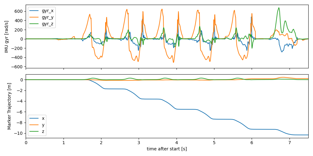
We plot the data of the heel marker (fcc) and the imu data of the insole sensor together to show that they are synchronised. Both data streams have the correct time axis, even though they are sampled at different rates (mocap is sampled with 100 hz, and IMU with 204.8). Keep that in mind, when working with the data without an index (e.g. after converting to numpy arrays).
To better visualize the data we “normalize” the mocap data by subtracting the first position. This way we can clearly see the individual strides.
fig, axes = plt.subplots(2, 1, sharex=True, figsize=(10, 5))
imu_data["l_insole"].filter(like="gyr").plot(ax=axes[0])
mocap_traj["l_fcc"].sub(mocap_traj["l_fcc"].iloc[0]).plot(ax=axes[1])
axes[0].set_xlim(0, 7.5)
axes[0].set_ylabel("IMU gyr [rad/s]")
axes[1].set_ylabel("Marker Trajectory [m]")
fig.tight_layout()
fig.show()
Like before we have access to the segmented strides (however, only cut for the respective region).
segmented_stride_labels = datapoint.segmented_stride_list_["left"]
segmented_stride_labels.head()
We can also access the labels for IC and TC. Even though we used the hand labeled strides as regions of interest for segmentation, we can see that the start and end labels of the mocap event strides and the hand labeled strides are not identical. This is because the event list is provided in the samples of the motion capture data, while the hand labeled strides are provided in the samples of the IMU data.
event_labels = datapoint.mocap_events_["left"]
event_labels.head()
To avoid errors in potential conversions between the two domains (mocap/IMU), we provide the
convert_with_padding methods to convert the event list.
(To understand why the method is called ..._with_padding, see the section below).
event_labels_in_imu = datapoint.convert_events_with_padding(event_labels, from_time_axis="mocap", to_time_axis="imu")
event_labels_in_imu.head()
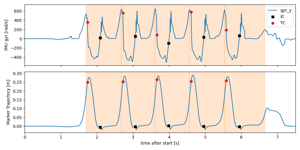
Now you can see, that the start and end labels are (almost) identical. Remaining differences are due to rounding errors. This is not ideal, but should not affect typical analysis.
Below we plotted the segmented strides and the IC and TC labels onto the gyr-y axis and the mocap z-axis (foot lift).
fig, axes = plt.subplots(2, 1, sharex=True, figsize=(10, 5))
gyr_y = imu_data["l_insole"]["gyr_y"]
norm_mocap_z = mocap_traj["l_fcc"].sub(mocap_traj["l_fcc"].iloc[0])["z"]
gyr_y.plot(ax=axes[0])
norm_mocap_z.plot(ax=axes[1])
event_labels_in_mocap = event_labels
event_labels_times = datapoint.convert_events_with_padding(event_labels, from_time_axis="mocap", to_time_axis="time")
event_labels_in_imu = datapoint.convert_events_with_padding(event_labels, from_time_axis="mocap", to_time_axis="imu")
for i, s in event_labels_times.iterrows():
    axes[0].axvspan(s["start"], s["end"], alpha=0.2, color="C1")
    axes[1].axvspan(s["start"], s["end"], alpha=0.2, color="C1")
axes[0].scatter(
    event_labels_times["ic"],
    gyr_y.iloc[event_labels_in_imu["ic"]],
    marker="s",
    color="k",
    zorder=10,
    label="IC",
)
axes[0].scatter(
    event_labels_times["tc"],
    gyr_y.iloc[event_labels_in_imu["tc"]],
    marker="o",
    color="C3",
    zorder=10,
    label="TC",
)
axes[1].scatter(
    event_labels_times["ic"],
    norm_mocap_z.iloc[event_labels_in_mocap["ic"]],
    marker="s",
    color="k",
    zorder=10,
    label="IC",
)
axes[1].scatter(
    event_labels_times["tc"],
    norm_mocap_z.iloc[event_labels_in_mocap["tc"]],
    marker="o",
    color="C3",
    zorder=10,
    label="TC",
)

axes[0].legend()
axes[0].set_xlim(0, 7.5)
axes[0].set_ylabel("IMU gyr [rad/s]")
axes[1].set_ylabel("Marker Trajectory [m]")
fig.tight_layout()
fig.show()
Data padding#
One issue that you might run into when working with the mocap version of the dataset is that the start of the test
(which is used to cut the signal) is right at the beginning of the movement.
This means for algorithms that require a certain resting period (e.g. to do a gravity alignment) might not work well.
Therefore, we provide a data_padding_s parameter that will load that amount of seconds before and after the
actual test.
On the time axis, we assign negative time stamps to all the padded values that are before the actual test start. This ensures that the time axis of the IMU data and the mocap data are still aligned, even tough no mocap data exists in the padded region.
dataset = SensorPositionComparison2019Mocap(
    memory=Memory("../.cache"),
    data_padding_s=3,
)
datapoint = dataset[0]
imu_data = datapoint.data
mocap_traj = datapoint.marker_position_
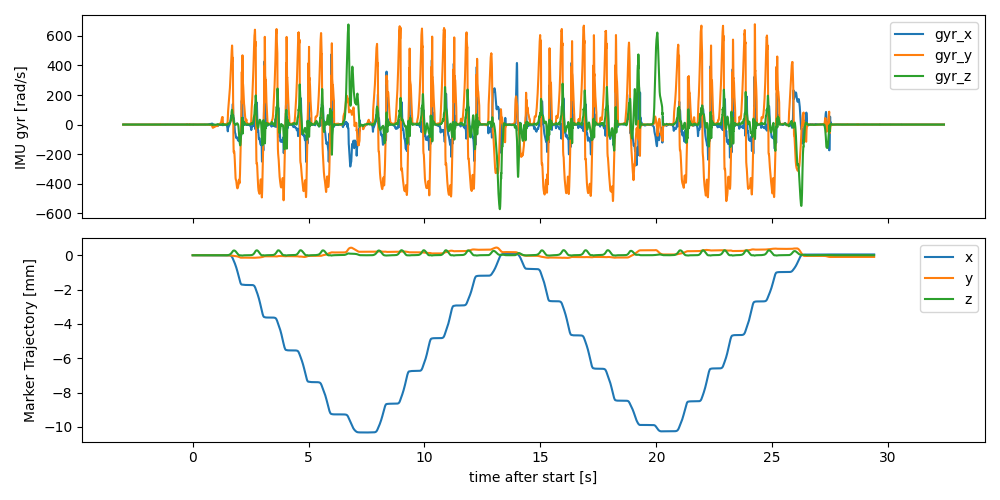
We can see that the data is now padded with 3 seconds before and after the test, however no mocap samples exist in these regions.
fig, axes = plt.subplots(2, 1, sharex=True, figsize=(10, 5))
imu_data["l_insole"].filter(like="gyr").plot(ax=axes[0])
mocap_traj["l_fcc"].sub(mocap_traj["l_fcc"].iloc[0]).plot(ax=axes[1])
axes[0].set_ylabel("IMU gyr [rad/s]")
axes[1].set_ylabel("Marker Trajectory [mm]")
fig.tight_layout()
fig.show()
While the time axis of the IMU data is still aligned with the mocap data, care needs to be taken when it comes to
the event data.
Only events/labels provided with IMU samples (or with a time axis) respect the padding correctly.
For example, the segmented_stride_list is provided with in IMU samples, so it is padded correctly.
- Note: The strides that are included in the segmented stride list will not change, if you increase the padding!
This means if you increase the padding so that strides outside the selected gait tests are part of the signal, they will not be included in the segmented stride list.
segmented_stride_labels = datapoint.segmented_stride_list_["left"]
segmented_stride_labels.head()
However, to correctly transform it to the time domain, you need to manually add the padding time.
To avoid erros, we provide the convert_with_padding method that does this for you.
segmented_stride_labels_time = datapoint.convert_events_with_padding(
    segmented_stride_labels, from_time_axis="imu", to_time_axis="time"
)
segmented_stride_labels_time.head()
Values provided in mocap samples, don’t have any padding applied.
However, for the like with the segmented_stride_list, you can use convert_with_padding to transform them to IMU
samples with correct padding.
First no padding, mocap samples
event_labels_in_mocap = datapoint.mocap_events_["left"]
event_labels_in_mocap.head()
In IMU samples with padding:
event_labels_in_imu = datapoint.convert_events_with_padding(
    event_labels_in_mocap, from_time_axis="mocap", to_time_axis="imu"
)
event_labels_in_imu.head()
And in time (seconds) with padding: Below you can see that the first event is now after 4 seconds, indicating that the signal is correctly padded.
event_labels_times = datapoint.convert_events_with_padding(
    event_labels_in_mocap, from_time_axis="mocap", to_time_axis="time"
)
event_labels_times.head()
Other coordinate transformations#
For reference, here are visual representations for the coordinate systems transforms used for all the foot sensors.


Total running time of the script: ( 0 minutes 16.035 seconds)
Estimated memory usage: 690 MB