PyShoe2019 - Indoor Navigation with foot-mounted inertial sensors#

The PyShoe dataset [1] contains multiple trials with spatial reference for longer trials. This makes it perfect to benchmark trajectory reconstruction algorithms. However, it does not contain any temporal marker or stride reference.

General information#

The dataset was recorded with a LORD MicroStrain 3DM-GX5-25 IMU sensor. A single IMU node was attached on the top of the right shoe.

On loading, we transform the data to the coordinate system of the gaitmap coordinate system as shown below

coordinate system definition

The data is split into three parts:

  • Vicon: Individual trials recorded with a Vicon motion capture system as reference

  • Hallway: Multiple longer walking/running trials recorded with specific landmarks as positional reference along the trial

  • Stairs: Multiple trials from a single participant recorded with a stair climbing task

For each part of the data we provide a separate dataset class.

Warning

For this example to work, you need to have a global config set containing the path to the dataset. Check the README.md for more information.

Vicon Dataset#

First we will create a simple instance of the dataset class.

from gaitmap_datasets.pyshoe_2019 import PyShoe2019Vicon

dataset = PyShoe2019Vicon()
dataset

PyShoe2019Vicon [56 groups/rows]

trial
0 2017-12-15-18-01-18
1 2017-11-27-11-12-18
2 2017-11-27-11-13-41
3 2017-11-22-11-22-46
4 2017-11-22-11-49-29
5 2017-11-22-11-44-47
6 2017-12-15-17-59-19
7 2017-11-22-11-22-03
8 2017-11-22-11-38-45
9 2017-11-27-11-11-24
10 2017-11-27-11-24-07
11 2017-11-22-11-36-45
12 2017-11-22-11-39-47
13 2017-11-22-11-51-23
14 2017-11-22-11-27-30
15 2018-02-09-11-18-04
16 2017-11-27-11-13-10
17 2018-02-09-11-32-01
18 2017-11-27-11-14-03
19 2018-02-09-11-16-53
20 2018-02-09-11-19-39
21 2017-11-27-11-19-16
22 2017-12-15-17-59-50
23 2018-02-22-10-10-56
24 2017-11-22-11-48-35
25 2017-11-22-11-49-03
26 2017-11-27-11-18-11
27 2017-11-22-11-52-02
28 2017-11-27-11-17-28
29 2017-11-27-11-22-22
30 2018-02-09-11-22-01
31 2018-02-22-10-09-36
32 2017-11-22-11-37-47
33 2017-11-22-11-28-39
34 2017-11-22-11-28-03
35 2017-11-27-11-12-44
36 2017-11-22-11-26-46
37 2017-12-15-18-03-05
38 2017-11-27-11-23-18
39 2017-11-22-11-35-59
40 2017-12-15-18-01-51
41 2017-11-22-11-25-20
42 2017-11-27-11-25-12
43 2017-11-22-11-26-05
44 2017-11-22-11-30-14
45 2017-12-15-18-00-40
46 2017-11-27-11-11-53
47 2017-11-27-11-14-52
48 2017-11-22-11-40-44
49 2018-02-22-10-10-29
50 2017-11-22-11-50-42
51 2017-12-15-18-00-13
52 2017-11-22-11-23-25
53 2018-02-09-11-29-43
54 2017-12-15-18-02-28
55 2018-02-22-10-08-52


Based on the index you can select individual trials. Note, that some of the trials contain running/shuffling or backward walking. However, the dataset authors do not provide a label for that (utiasSTARS/pyshoe#11). If it is important to you to only consider trials containing movements of a specific type, you need to manually check the raw data and guess based on that.

trial = dataset.get_subset(trial="2017-11-22-11-22-03")

When we have selected a single trial, we can access the data. The data is stored in a pandas DataFrame, where each row corresponds to a single time step. Note, that the dataset only contains data from a single IMU attached to the right shoe. We still provide the data as a “nested” dataframe, where the outermost level corresponds to the foot.

imu_data = trial.data
imu_data
sensor right_sensor
axis acc_x acc_y acc_z gyr_x gyr_y gyr_z
time [s]
0.005191 -2.781892 -0.299658 9.352644 0.227405 -0.706740 0.485781
0.010160 -2.841245 -0.315210 9.339815 0.207448 0.063552 -0.090120
0.015174 -2.821833 -0.278027 9.385390 0.940303 0.466289 0.586400
0.020134 -2.854676 -0.298270 9.383124 0.341406 0.091222 0.328716
0.025084 -2.879035 -0.242348 9.389574 0.631465 0.462962 -0.334062
... ... ... ... ... ... ...
32.429850 -2.601544 -0.585042 9.421066 0.256404 -0.408682 0.334698
32.434979 -2.639347 -0.582814 9.398733 0.384274 0.751468 -0.036125
32.440075 -2.631892 -0.585243 9.393909 -1.039280 0.817331 -0.120867
32.444980 -2.669842 -0.585144 9.419175 0.161355 0.875428 -0.333420
32.449892 -2.620204 -0.579081 9.422248 -0.996577 1.384654 0.173012

6490 rows × 6 columns


The mocap marker data is also stored in a pandas DataFrame and the marker is placed directly on the sensor.

mocap_data = trial.marker_position_
mocap_data
sensor right_sensor
direction x y z
time [s]
0.005191 -27.581452 63.427551 125.979013
0.010160 -27.600539 63.421317 126.002191
0.015174 -27.600539 63.421317 126.002191
0.020134 -27.599742 63.405152 125.977403
0.025084 -27.555421 63.640739 126.079271
... ... ... ...
32.429850 -34.302266 2.244311 122.834868
32.434979 -34.333242 2.226604 122.793186
32.440075 -34.323351 2.185406 122.843320
32.444980 -34.325223 2.169762 122.815674
32.449892 -34.279827 2.199983 122.776791

6490 rows × 3 columns


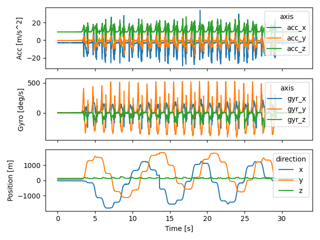
Both data types are recorded at 200 Hz and are synchronized. This means we can plot them in an aligned way without any modifications.

import matplotlib.pyplot as plt

fig, axs = plt.subplots(3, 1, sharex=True)
imu_data["right_sensor"].filter(like="acc").plot(ax=axs[0])
imu_data["right_sensor"].filter(like="gyr").plot(ax=axs[1])
mocap_data["right_sensor"].plot(ax=axs[2])
axs[2].set_xlabel("Time [s]")
axs[2].set_ylabel("Position [m]")
axs[1].set_ylabel("Gyro [deg/s]")
axs[0].set_ylabel("Acc [m/s^2]")

fig.tight_layout()
fig.show()
pyshoe 2019

Hallway Dataset#

First we will create a simple instance of the dataset class. We can see that the dataset contains trials from multiple participants with the three trial types (walking, running, combined).

from gaitmap_datasets.pyshoe_2019 import PyShoe2019Hallway

dataset = PyShoe2019Hallway()
dataset

PyShoe2019Hallway [38 groups/rows]

participant type trial
0 p3 walk 2018-04-10-15-25-02
1 p3 walk 2018-04-10-15-18-40
2 p2 walk 2018-04-11-19-42-05
3 p2 walk 2018-04-11-19-49-39
4 p4 walk 2018-04-11-15-26-05
5 p4 walk 2018-04-11-15-20-30
6 p1 walk 2018-04-11-10-46-37
7 p1 walk 2018-04-11-10-39-53
8 p0 walk 2018-04-10-14-04-36
9 p0 walk 2018-04-07-15-39-07
10 p0 walk 2018-04-07-15-42-42
11 p3 comb 2018-04-10-15-37-06
12 p3 comb 2018-04-10-15-31-18
13 p2 comb 2018-04-11-20-02-58
14 p2 comb 2018-04-11-19-56-12
15 p4 comb 2018-04-11-15-36-03
16 p4 comb 2018-04-11-15-31-34
17 p1 comb 2018-04-11-10-59-05
18 p1 comb 2018-04-11-10-53-28
19 p0 comb 2018-04-09-10-53-15
20 p0 comb 2018-04-09-10-24-18
21 p0 comb 2018-04-09-11-03-28
22 p0 comb 2018-04-09-11-07-05
23 p0 comb 2018-04-09-10-56-09
24 p0 comb 2018-04-09-11-00-12
25 p3 run 2018-04-10-15-22-44
26 p3 run 2018-04-10-15-29-20
27 p2 run 2018-04-11-19-47-16
28 p2 run 2018-04-11-19-54-02
29 p4 run 2018-04-11-15-24-01
30 p4 run 2018-04-11-15-29-42
31 p1 run 2018-04-11-10-51-02
32 p1 run 2018-04-11-10-44-34
33 p0 run 2018-04-09-10-31-05
34 p0 run 2018-04-09-10-21-01
35 p0 run 2018-04-16-13-46-32
36 p0 run 2018-04-16-11-37-48
37 p0 run 2018-04-10-14-08-29


We can select arbitrary subsets of the data. For example, we can select all combined (running+walking) trials of a specific participant.

subset = dataset.get_subset(participant="p1", type="comb")
subset

PyShoe2019Hallway [2 groups/rows]

participant type trial
0 p1 comb 2018-04-11-10-59-05
1 p1 comb 2018-04-11-10-53-28


When we have selected a single trial, we can access the data.

trial = subset[0]
trial

PyShoe2019Hallway [1 groups/rows]

participant type trial
0 p1 comb 2018-04-11-10-59-05


We can access the IMU data as before.

imu_data = trial.data
imu_data
sensor right_sensor
axis acc_x acc_y acc_z gyr_x gyr_y gyr_z
time [s]
0.005149 -4.590975 4.374997 7.437768 0.448315 0.189880 0.417674
0.010360 -4.544281 4.373245 7.510326 0.299517 0.177923 0.289822
0.015975 -4.540386 4.391929 7.457896 0.233851 0.169668 0.185347
0.016173 -4.584002 4.351857 7.462299 0.215938 0.148307 0.105725
0.020918 -4.611207 4.384323 7.468820 0.053287 0.018772 0.133610
... ... ... ... ... ... ...
287.435578 -4.865076 4.539700 7.210635 0.286556 0.288634 0.009507
287.440897 -4.839256 4.545354 7.210913 0.283526 0.272317 0.029565
287.445866 -4.893078 4.548808 7.172363 0.186191 0.141298 0.113512
287.451062 -4.847052 4.542258 7.177924 0.157011 0.151041 0.118710
287.456193 -4.847890 4.602775 7.157774 0.136902 0.098196 0.151553

57491 rows × 6 columns


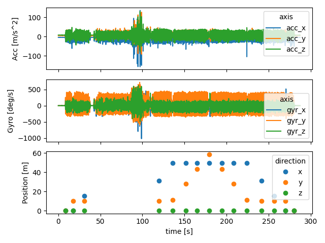
The reference position is only provided for individual points along the trial.

reference = trial.position_reference_
reference
sensor right_sensor
direction x y z
time [s]
8.282805 0.000000 0.000000 0.000000
17.575982 -0.028122 10.070310 0.045138
31.179760 15.212801 10.027737 0.015693
119.851323 31.064606 10.009687 0.018403
136.169768 49.617972 11.036337 0.063391
151.923731 49.586710 28.185467 0.085439
165.107195 49.586710 43.048866 0.140000
179.220718 49.586710 58.590090 0.221820
194.378116 49.586710 43.048866 0.140000
208.105069 49.586710 28.185467 0.085439
224.395774 49.617972 11.036337 0.063391
241.569288 31.064606 10.009687 0.018403
256.481009 15.212801 10.027737 0.015693
269.811253 -0.028122 10.070310 0.045138
280.424826 0.000000 0.000000 0.000000


The index of the reference corresponds to timestamps in the IMU data. Hence, we can easily get the IMU data for the time points of the reference (or the position, once we have calculated it based on the IMU data).

sensor right_sensor
axis acc_x acc_y acc_z gyr_x gyr_y gyr_z
time [s]
8.282805 -4.496491 4.253400 7.412974 29.790430 32.970402 -9.761967
17.575982 -4.776118 4.659799 7.333980 -11.914205 0.801795 -8.811063
31.179760 -4.989060 4.365822 7.425811 8.321191 13.408360 -4.438745
119.851323 -4.807809 4.710577 7.425576 7.896716 11.902532 -5.582264
136.169768 -5.055169 3.813725 7.553582 3.564295 1.834236 2.327311
151.923731 -4.469937 4.358171 7.634457 2.966452 10.305689 -7.623919
165.107195 -4.533692 4.353279 7.669889 7.478448 7.827342 -0.394508
179.220718 -4.839216 4.395577 7.574844 -8.672488 -4.053169 -4.078138
194.378116 -4.372919 4.784847 7.529003 -5.934276 6.279567 -7.534290
208.105069 -4.657144 4.509208 7.326108 -0.939665 8.969255 -6.471187
224.395774 -4.782296 4.156237 7.608356 -5.762303 5.037054 -8.894644
241.569288 -4.496109 4.155525 7.856090 3.373532 6.504419 -3.857418
256.481009 -4.659771 4.991015 7.000360 15.608949 52.334545 -30.418329
269.811253 -6.076867 1.637763 7.649946 -38.121038 -7.439257 -18.199075
280.424826 -4.531105 5.201338 6.754158 -1.063248 -1.165655 3.970324


Below we plot all the data together.

fig, axs = plt.subplots(3, 1, sharex=True)
imu_data["right_sensor"].filter(like="acc").plot(ax=axs[0])
imu_data["right_sensor"].filter(like="gyr").plot(ax=axs[1])
reference["right_sensor"].plot(ax=axs[2], style="o")
axs[2].set_ylabel("Position [m]")
axs[1].set_ylabel("Gyro [deg/s]")
axs[0].set_ylabel("Acc [m/s^2]")

fig.tight_layout()
fig.show()
pyshoe 2019

Stairs Dataset#

The dataset contains trails of a participant walking different number of levels of stairs in starcase. For each number of stairs one trail exists that starts with the participant walking down and then back up ( first_direction="down") and one trial that starts with the participant walking up and then back down ( first_direction="up").

First we will create a simple instance of the dataset class.

from gaitmap_datasets.pyshoe_2019 import PyShoe2019Stairs

dataset = PyShoe2019Stairs()
dataset

PyShoe2019Stairs [8 groups/rows]

n_levels first_direction trial
0 8 up 2018-08-11-13-31-07-up-8
1 4 up 2018-08-11-14-10-37-up-4
2 4 down 2018-08-11-14-27-26-down-4
3 2 up 2018-08-11-14-15-16-up-2
4 8 down 2018-08-11-14-20-21-down-8
5 6 down 2018-08-11-14-24-15-down-6
6 6 up 2018-08-11-14-07-34-up-6
7 2 down 2018-08-11-14-31-07-down-2


We can simply select either the trials starting with going down the up or down trials.

subset = dataset.get_subset(first_direction="down")
subset

PyShoe2019Stairs [4 groups/rows]

n_levels first_direction trial
0 4 down 2018-08-11-14-27-26-down-4
1 8 down 2018-08-11-14-20-21-down-8
2 6 down 2018-08-11-14-24-15-down-6
3 2 down 2018-08-11-14-31-07-down-2


When we have selected a single trial, we can access the data.

trial = subset.get_subset(n_levels="6")
trial

PyShoe2019Stairs [1 groups/rows]

n_levels first_direction trial
0 6 down 2018-08-11-14-24-15-down-6


We can access the IMU data as before.

imu_data = trial.data
imu_data
sensor right_sensor
axis acc_x acc_y acc_z gyr_x gyr_y gyr_z
time [s]
0.005208 -0.822558 4.476494 8.648929 -0.480159 0.368659 0.008838
0.010548 -0.825832 4.495879 8.630640 -0.567628 0.320375 0.086155
0.015669 -0.835436 4.468421 8.603162 -0.546395 0.376312 0.091157
0.020823 -0.832943 4.481061 8.640306 -0.651113 0.359915 0.039598
0.025965 -0.793898 4.492451 8.655291 -0.671351 0.438643 0.178911
... ... ... ... ... ... ...
111.475393 -0.910722 4.394284 8.681709 0.105375 -0.058603 0.083301
111.480583 -0.941793 4.378661 8.652824 0.122981 -0.003054 -0.005066
111.485680 -0.963584 4.405440 8.653285 0.081241 -0.085321 0.022283
111.490844 -0.924065 4.375131 8.686098 0.161671 -0.108651 0.012238
111.495891 -0.913383 4.400737 8.725246 0.071880 -0.117503 0.099150

22299 rows × 6 columns


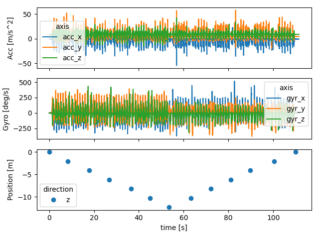
As with the hallway dataset the reference position is only provided for individual points along the trial. Further, as the reference is derived from the stair geometry, reference only exist for the z-axis.

reference = trial.position_reference_
reference
sensor right_sensor
direction z
time [s]
0.005208 0.000
8.346160 -2.057
17.920212 -4.114
26.741772 -6.171
36.641167 -8.228
45.039189 -10.285
53.406863 -12.342
63.202737 -10.285
72.240978 -8.228
81.027286 -6.171
89.735355 -4.114
100.411463 -2.057
109.918265 0.000


Below we plot all the data together.

fig, axs = plt.subplots(3, 1, sharex=True)
imu_data["right_sensor"].filter(like="acc").plot(ax=axs[0])
imu_data["right_sensor"].filter(like="gyr").plot(ax=axs[1])
reference["right_sensor"].plot(ax=axs[2], style="o")
axs[2].set_ylabel("Position [m]")
axs[1].set_ylabel("Gyro [deg/s]")
axs[0].set_ylabel("Acc [m/s^2]")

fig.tight_layout()
fig.show()
pyshoe 2019

Total running time of the script: ( 0 minutes 11.348 seconds)

Estimated memory usage: 30 MB

Gallery generated by Sphinx-Gallery