Note
Click here to download the full example code
EgaitParameterValidation2013 - A Stride Parameter validation dataset#
The EgaitParameterValidation2013 dataset allows access to the parameter validation dataset recorded for the EGait system. It contains multiple short walks recorded by two foot worn IMU sensors and a GaitRite carpet as reference. Unfortunately, the Gaitrite and the IMU sensors are not synchronized. To solve this, the IMU-data was cut to the strides that are expected to be on the GaitRite carpet by counting the number of strides performed in both systems (see original publication for more info).
General information#
The dataset was recorded with Shimmer 2R sensors. In these IMU nodes, the coordinate systems of the accelerometer and the gyroscope are different.
In the version provided in this dataset, we fix this by transforming the gyroscope data to the accelerometer coordinate system and then transform the combined data to the coordinate system of the gaitmap coordinate system.
Note
In the instructions provided with the dataset, the conversation of the gyroscope data is not mentioned, but was handled by the authors as part of their data processing pipeline.
In the following we will show how to interact with the dataset and how to make sense of the reference information.
Warning
For this example to work, you need to have a global config set containing the path to the dataset.
Check the README.md for more information.
import pandas as pd

from gaitmap_datasets import EgaitParameterValidation2013
First we will create a simple instance of the dataset class. We can see that it contains a single recording per participant for 101 participants.
For this example, we will select the data of a single participant.
subset = dataset.get_subset(participant="P115")
subset
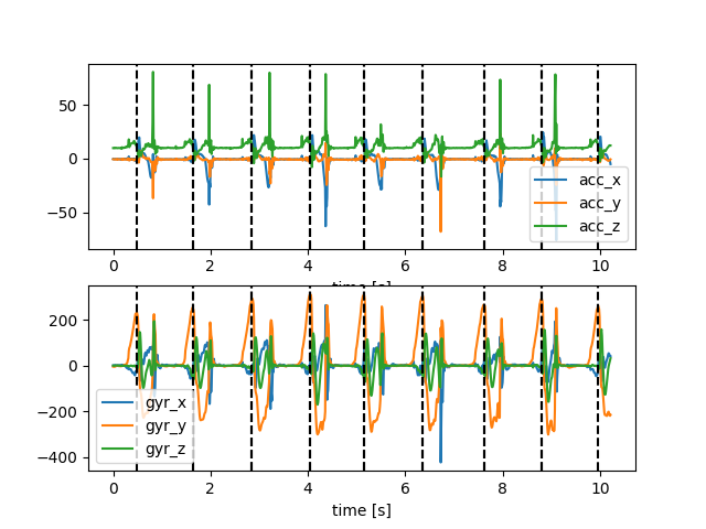
And simply plot the gait data and the manually labeled stride borders.
import matplotlib.pyplot as plt

imu_data = subset.data
segmented_stride_list = subset.segmented_stride_list_

_, axs = plt.subplots(2, 1)
foot = "right_sensor"
imu_data[foot].filter(like="acc").plot(ax=axs[0])
imu_data[foot].filter(like="gyr").plot(ax=axs[1])

for i, s in segmented_stride_list[foot].iterrows():
    s /= subset.sampling_rate_hz
    axs[0].axvline(s["start"], color="k", linestyle="--")
    axs[0].axvline(s["end"], color="k", linestyle="--")
    axs[1].axvline(s["start"], color="k", linestyle="--")
    axs[1].axvline(s["end"], color="k", linestyle="--")

plt.show()

We can see that the IMU data is cut right in the middle of the movement to only contain the strides that were also detected by the GaitRite system. However, the GaitRite system defines strides from initial contact (IC) to initial contact (IC), while the manual stride annotations define the strides from a maximum in the gyro-signal to the next (see image above).
This means that even-though the signal should contain the same strides as the reference, they don’t line up. When we compare the number of manual strides with the number of parameterized strides, we can see that there is always one stride less in the parameterized data.
{'left_sensor':       stride_length  stride_time  stance_time  swing_time
s_id
0           0.62577        1.167        0.867       0.300
1           0.70900        1.208        0.850       0.358
2           0.69898        1.167        0.884       0.283
3           0.80049        1.142        0.834       0.308
4           0.79072        1.191        0.867       0.324
5           0.75001        1.250        0.892       0.358
6           0.64322        1.200        0.909       0.291
7           0.60007        1.134        0.751       0.383, 'right_sensor':       stride_length  stride_time  stance_time  swing_time
s_id
0           0.64356        1.150        0.842       0.308
1           0.76768        1.250        0.909       0.341
2           0.73267        1.142        0.850       0.292
3           0.77054        1.133        0.808       0.325
4           0.77210        1.233        0.875       0.358
5           0.66853        1.217        0.909       0.308
6           0.61293        1.133        0.884       0.249}
parameters["left_sensor"].shape
(8, 4)
segmented_stride_list["left_sensor"].shape
(9, 2)
This is caused by the different stride definitions, as explained above.
To align them, we need to first detect relevant stride events (i.e. at least the IC) from the IMU signal. We should ensure that exactly one IC is detected per segmented stride. Then we can use this information to create a new stride list (from one IC to the next), that should align with the parameterized strides from the GaitRite system.
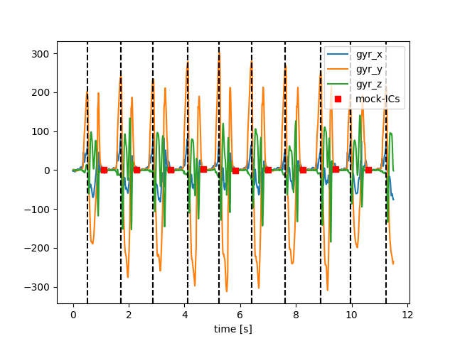
As this library includes no method to detect ICs, we will mock this to demonstrate the approach. We simply assume that the IC is always in the center of segmented stride.
foot = "left_sensor"

mock_gait_events = segmented_stride_list[foot].copy()
mock_gait_events["ic"] = mock_gait_events["start"] + (mock_gait_events["end"] - mock_gait_events["start"]) // 2
Let’s plot the mock gait events.
_, ax = plt.subplots(1, 1)
imu_data[foot].filter(like="gyr").plot(ax=ax)

for i, s in segmented_stride_list[foot].iterrows():
    s /= subset.sampling_rate_hz
    ax.axvline(s["start"], color="k", linestyle="--")
    ax.axvline(s["end"], color="k", linestyle="--")

ics = mock_gait_events["ic"] / subset.sampling_rate_hz
imu_data[foot]["gyr_y"].loc[ics].plot(ax=ax, color="r", style="s", label="mock-ICs")
ax.legend()
plt.show()

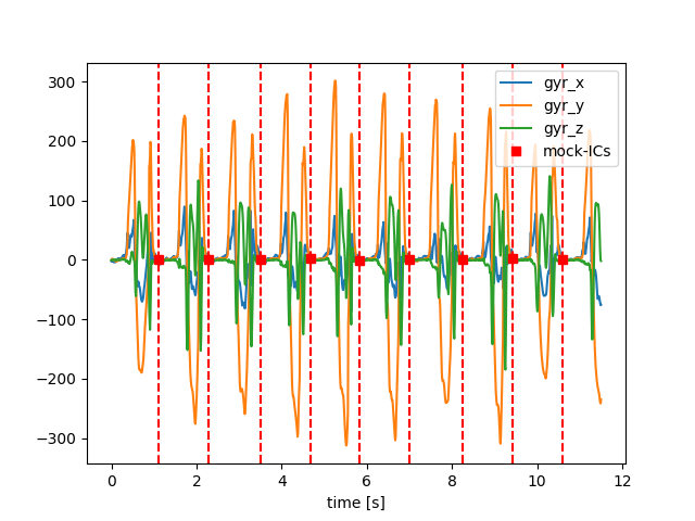
Using these mock ICs, we can create a new stride list where each stride starts and ends at the “detected” ICs.
new_stride_list = mock_gait_events[["ic"]].copy()
new_stride_list["start"] = new_stride_list["ic"]
new_stride_list["end"] = new_stride_list["ic"].shift(-1)
new_stride_list = new_stride_list.dropna().astype(int)
new_stride_list
_, ax = plt.subplots(1, 1)
imu_data[foot].filter(like="gyr").plot(ax=ax)

for i, s in new_stride_list.iterrows():
    s /= subset.sampling_rate_hz
    ax.axvline(s["start"], color="r", linestyle="--")
    ax.axvline(s["end"], color="r", linestyle="--")

ics = mock_gait_events["ic"] / subset.sampling_rate_hz
imu_data[foot]["gyr_y"].loc[ics].plot(ax=ax, color="r", style="s", label="mock-ICs")
ax.legend()
plt.show()

This new stride list has the same number of strides as the parameterized strides and the strides should roughly line up. This means we can use the parameterized strides to evaluate calculated stride parameters.
Here, we will calculate a “mock” stride time.
imu_parameters = pd.DataFrame(
    {"stride_time": (new_stride_list["end"] - new_stride_list["start"]) / subset.sampling_rate_hz},
    index=new_stride_list.index,
)
imu_parameters
With that we can calculate the error of our stride parameters against the reference.
error = (imu_parameters["stride_time"] - parameters[foot]["stride_time"]).abs().rename("abs. Stride Time Error [s]")
error
s_id
0    0.014641
1    0.006828
2    0.014641
3    0.010344
4    0.009359
5    0.009766
6    0.037891
7    0.047641
Name: abs. Stride Time Error [s], dtype: float64
Similarly to this approach other parameters can be calculated and compared. Just keep in mind, that you always need to first detect either ICs (or other gait events) within the segmented strides and then shift the stride definition before comparing the parameters.
Total running time of the script: ( 0 minutes 3.055 seconds)
Estimated memory usage: 8 MB